Are you ready for another Excel formula challenge from the Modeloff 2013 group challenge? Question #2 requires some knowledge about array formulas and just some flat out formula building creativity. Many thanks to Dan Mayoh for providing the answers to us. Dan recently launched his consulting business called Fintega Pty Ltd; the site is still under construction but if you are in the market for some finance consulting, send an e-mail to dan@fintega.com. Test your Excel skills again with this week’s challenge!

The Challenge

In case you missed the ground rules for the group challenge, read the first post in this series of Excel formula challenges. Similar to last week, you have a range of blue cells where you need to enter in the solution formula:

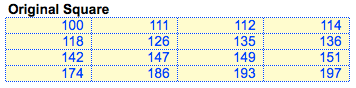
There is also a range of numbers next to the blue cells which you must use in the challenge:

The Objective: Write a formula to rotate the values in the 4*4 square through 180 degrees.

All the numbers need to be “flipped” along both the X-axis and Y-axis. Here is what the final table of answers should look like in the blue cells:

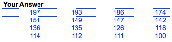
Here is a side-by-side comparison between the original range of numbers and what the final output should look like in the blue cells:

Give it a shot! Download this file that represents the data discussed above and see if you can create the formula!

The Solution

When I first looked at this challenge, I knew it involved using array formulas. For those not familiar with array formulas, here is a good guide from Mr. Excel that explains how array formulas work and why they are useful. I was seriously stumped by the question, and struggled to figure out how to “flip” the numbers in an automated way.

The solution involves using the simple SUM() function in an array formula in an elegant fashion. The final formula consists of 33 characters:

SUM($E$18:$H$21*(B15:E18=$E$18))

This is the formula you enter in the first cell of the blue cells in the array format (by pressing CTRL+SHIFT+ENTER) after you’ve written the formula. You then copy over to all the cells in the range to yield the final table of answers.

The Explanation

This formula compares two ranges of values through an array formula. If you simply entered the formula as is and pressed ENTER, you would get a #VALUE error in the cell since you are supplying the SUM() function with a conditional statement.

Let’s back up and see how array formulas work in the context of this solution. Let’s analyze the $E$18:$H$21 portion of the formula. This is simply the range of numbers we need to flip to get our solution. By entering this formula as an array formula, this specific portion of the formula returns an array of values like this:

{100, 111, 112, 114, 118, 126, 135, 136, 142, 147, 149, 151, 174, 186, 193, 197}

The B15:E18=$E$18 portion of the formula is a little different since we are testing a condition against an array of values. In this case, we are testing each value in the B15:E18 range to see if that value matches the value in $E$18. The B15:E18 range of values returns an array that is mostly empty except for the last value:

{"", "", "", "", "", "", "", "", "", "", "", "", "", "", "", 100}

The reason why there are so many blanks is simple. The range B15:E18 is what I like to call a “dummy” range since it’s created mostly to help with making the final formula work. Cells B15, C15, D15, etc. are all empty in the worksheet. The B15:E18=$E$18 condition actually returns an array of TRUE and FALSE values, or 0s and 1st based on whether or not the values in the B15:E18 range equal cell $E$18, or 100. Thus, the array of values returned from testing B15:E18 with the value 100 is this:

{FALSE, FALSE, FALSE, FALSE, FALSE, FALSE, FALSE, FALSE, FALSE, FALSE, FALSE, FALSE, FALSE, FALSE, FALSE, TRUE}

Mathematically, this array actually looks like this:

{0, 0, 0, 0, 0, 0, 0, 0, 0, 0, 0, 0, 0, 0, 0, 1}

So now we have two arrays: one with the values in $E$18:$E$21 and one with the 0s and 1s from testing range B15:E18 with the value 100. The “*” in the formula multiplies the first array by the second array. The product of this is…you guessed it! Another array of 16 values.

{0, 0, 0, 0, 0, 0, 0, 0, 0, 0, 0, 0, 0, 0, 0, 197}

This array above is what’s returned from $E$18:$H$21*(B15:E18=$E$18) when entered as an array formula. Why is the last value 197? Remember the first array $E$18:$H$21 consists of all the numbers in the original square. When we multiply all those numbers with the second array with the 0s and 1s, the first 15 numbers in the resulting array are 0 (due to the FALSE values) and the last number 197 gets multiplied by 1 (the only TRUE value in the second array). The SUM() function simply adds everything up in the array together which results the value 197. This is the correct number in the top left of the blue answer cells.

The real magic occurs when you copy this formula to all the cells in the blue answer cells. Let’s look at the formula in cell K19 of the answer cells:

SUM($E$18:$H$21*(C16:F19=$E$18))

You’ll notice that the only thing that changed about this array formula is the relative range C16:F19. All the other referenced cells are absolute references. As you copy the formulas over to the other cells in the answer table, the “dummy” range of cells begins to shift to help create this “flipped” axis of numbers. If we break down the two arrays that are multiplied together, you’ll see how this works. $E$18:$H$21 remains the same:

{100, 111, 112, 114, 118, 126, 135, 136, 142, 147, 149, 151, 174, 186, 193, 197}

When we test C16:F19 against $E$19 now, the C16:F19 dummy range starts to include some of the numbers in the original table of numbers. This effectively helps us “count” which position in the second array contains the TRUE value. The resulting array of C16:F19=$E$19 is:

{0, 0, 0, 0, 0, 0, 0, 0, 0, 0, 1, 0, 0, 0, 0, 0}

The 11th value in the above array is the TRUE value because that’s when the value in range C16:F19 equals 100. When we multiply this array of 0s and 1s with the original table of numbers, the resulting array is this:

{0, 0, 0, 0, 0, 0, 0, 0, 0, 0, 149, 0, 0, 0, 0, 0}

Of course, when we sum up the numbers in this array, the result is 149 which is the correct number in cell K149 of the blue answer cells.

Conclusion

There are two other formulas that deserve honorable mentions which we won’t go into detail about how they work, but they show how you can get creative in Excel to solve problems with different functions. Both of these formulas clock in at 35 characters:

INDEX(E18:H21,{4;3;2;1},{4,3,2,1})

OFFSET($E$18,21-ROW(),13-COLUMN())

The first formula is array-entered into all 16 cells in the blue answer cells simultaneously. The second formula is entered into the first cell of the answer table (Cell J18) and copied across and down to the rest of the cells in the range.

Were you able to come up with other solutions? How long did it take you to answer this question?