Dear Analyst #133: Find or check if a cell contains text from a list of values or partial matching text in a list (3 methods)

There are times when a problem nags at you like a pebble in your shoe. Even when you’re not working on the problem itself, you’re thinking about the problem which make it even worse. Rarely do I come across a Google Sheets/Excel task I cannot solve with formulas, but this one evaded my extensive knowledge (or lack thereof). The reason why this problem kept on nagging at me was because it felt like it should be easy to do. Like it was something I’ve solved before in the past. Or a data manipulation task that should be easy to solve. Yet, when I tried building out the solution, I couldn’t quite figure it out. Here’s a quick graphic showing the data question at hand:

Breaking down the problem of checking if cell value contains text from another list

Seems simple, right? I have a bunch of sentences in column A and a bunch of words in column C. I want to know if the sentences in column A contain any of the words in column C.

I faced this task at work a few weeks ago and the kicker was not only did I need to figure out if the sentence contained the word, but also return another column from that “List to check” (imagine another list of values in column D in the screenshot above that I want to return). Immediately, I thought about different permutations of VLOOKUP and SEARCH but quickly realized on their own or combined, these formulas wouldn’t to the trick.

If we break down the problem, what we really need to do is this:

Loop through each color in column C
Check to see if cell A2 contains any of the words in step #1
If it does, great! Return a TRUE or another column from the lookup list
Move to cell A3 and loop through all the colors again

Once we think through the steps involved, it starts to become a trickier problem. Again, I thought this problem would have a simple solution. It kept on nagging at me so I figured I should share the solution I came up with in this episode. The solution I’m showing below is in Google Sheets and the formulas are slightly different (actually easier) in Excel. Here’s the Google Sheet with the 3 methods I came up with after doing some research. This episode is also a YouTube tutorial if you prefer seeing the solution:

Method 1: Check if cell value contains text from list (partial match) and return TRUE or FALSE

This first method is actually the most important method to understand because it’s building block for methods #2 and #3 where we want to return another column from the lookup list. This is the actual dummy data from the Google Sheet we’ll be using to build out the formula for method #1:

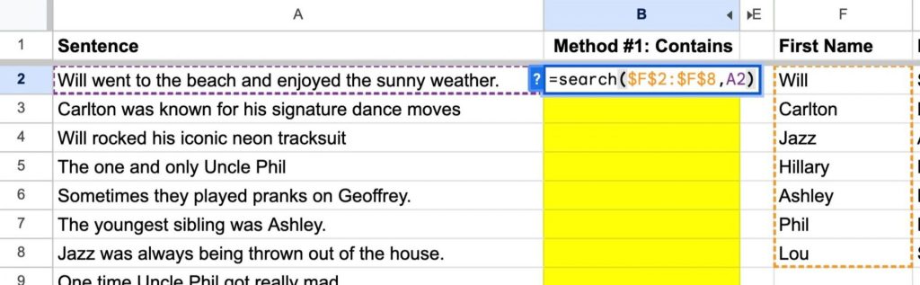
The ten sentences all contain the first name of a character from the TV show The Fresh Prince of Bel Air (one of the all-time greatest TV shows, of course). There are a list of first names of each character in column F. Some sentences do not contain a character from the list in column F. In column B, the goal is to write a formula that returns a TRUE or FALSE if the sentence in column A contains one of the first names in cells F2:F8. If you want to jump straight to the answer, the formula you write in cell B2 is this:

=OR(ARRAYFORMULA(ISNUMBER(ARRAYFORMULA(SEARCH($F$2:$F$8,A2)))))

If you’re using Excel (in Office 365), you can basically take out the ARRAYFORMULA in the formula or using CTRL+SHIFT+ENTER to enter the formula (if not using Office 365):

=OR(ISNUMBER(SEARCH($F$2:$F$8,A2)))

Utilizing the SEARCH function to find the name

To reiterate, this explanation only pertains to Google Sheets. In Excel, you have dynamic array formulas which change the behavior of functions like SEARCH and FIND. I won’t get into how dynamic array formulas in Excel work in this episode.

By itself, the SEARCH function gives you the position of a string of characters inside another string. In the first sentence, the result of doing SEARCH($F$2:$F$8,A2) gives you a result of 1 because Google Sheets finds the word “Will” in the sentence and “Will” starts at position 1 of the sentence:

Looping through each name with ARRAYFORMULA

If you drag the formula down, however, the formula breaks down. What it tries to do is compare each name with each sentence sequentially. So it tries to find “Carlton” in cell A3, “Jazz” in cell A4, etc. What we want the formula to do is search through all the names in each sentence and not just for whatever row the name appears on. That’s why we need to wrap the formula in an ARRAYFORMULA function which essentially goes through each value in $F$2:$F$8 and searches for the name in A2. So now our formula looks like this: ARRAYFORMULA(SEARCH($F$2:$F$8,A2)). In the screenshot below, I put the formula in cell B5 to better illustrate what’s happening:

We still see a bunch of #VALUE errors starting in cell B5 but in cell B10 we see the number 24. This formula still “spills” down starting from B5 similar to what happens in Excel. That’s because it’s going through all 7 names and looking for that name in cell A5. Google Sheets finds “Phil” in the sentence and the name appears in the 24th position in the sentence. That’s why the number 24 shows up in cell B10 even though it’s referencing cell B5. This is an important concept to grasp about spill and array formulas because the output is not one single value in a cell, but rather an array.

Getting a TRUE or FALSE value to handle the #VALUE error

The goal of method #1 is to get a TRUE or FALSE in column B. A quick function we can wrap our current function in is the ISNUMBER function. This function simply returns TRUE or FALSE if the output is a number. Let’s see what happens when we put the following formula in cell B2 and drag it down ISNUMBER(ARRAYFORMULA(SEARCH($F$2:$F$8,A2))):

It looks like it works because we see TRUE in cell B2 and in B4. Both of these sentences contain the name “Will.” But why does B3 say false? “Carlton” exists in the sentence. As you might’ve guessed, the ISNUMBER function is only searching for the name “Will” in each sentence as the cell reference in the SEARCH function changes. Recall that we got a bunch of #VALUE errors in the last formula. What we now need Google Sheets to do is go through each of these values in the array and ask if it’s a number:

So the result we want is something that looks like this:

What this actually looks like behind the scenes is {FALSE, FALSE, FALSE, FALSE, FALSE, TRUE, FALSE}. Therefore, we need to add in another ARRAYFORMULA to tell Google Sheets to inspect each value of the resulting array from the last section. So our formula looks like this now: =ARRAYFORMULA(ISNUMBER(ARRAYFORMULA(SEARCH($F$2:$F$8,A2)))). And the result is what we expect:

It’s still not correct because we just get a spilled formula showing whether or not cell A2 contains one of the first names.

Getting one TRUE or FALSE from the array

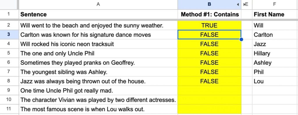
If we wrap this formula one more time in an OR function, the output is what we expect after we drag the formula down:

A way to visualize why the OR function works in this case is putting it in front of the array of TRUE and FALSEs from the previous section. This is what the array of TRUE and FALSEs looks like in cell A5 with “Phil”:

OR({FALSE, FALSE, FALSE, FALSE, FALSE, TRUE, FALSE})

As long as any of the values in the TRUE/FALSE array is TRUE, then the OR function returns one value: TRUE. If none of the values in the array are TRUE, then the one returned value is FALSE. So the OR function is a nice clean way of reducing the array down to one single TRUE or FALSE to show up in column B.

Method 2: Return another column from the list if the text is found in the cell with COUNTIF and XLOOKUP

We are now going to do what I was actually trying to do with my project at work. We don’t just want a TRUE or FALSE now. We want to return the last name from the list of names if the first name appears in the sentence. Instead of using SEARCH, we’ll be using the COUNTIF function as an alternative method to finding if 1) the first name exists in the sentence and 2) pulling back the last name. Going to skip a few steps and breakdown what this formula does: ARRAYFORMULA(COUNTIF(A2,"*"&$F$2:$F$8&"*")):

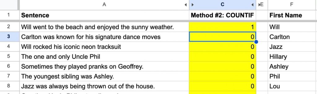
This is a unique way of using the COUNTIF function that I’ve never used before. Usually you’re using COUNTIF to see if a cell is greater or less than some value. In this case, we are using wild cards (the “*”) before the $F$2:$F:$8 reference. We’re telling Google Sheets to look for the word “Will” in the sentence regardless of what characters appear before or after the word as it appears in the sentence. The ARRAYFORMULA in front of COUNTIF also loops through each name in the list and looks for it in the sentence. If it finds the name mentioned, then it returns a 1 (counts the number times the word appears).

Similar to the SEARCH function, we get an array result but instead, it’s a bunch of 1s and 0s. Instead of wrapping this formula in another ARRAYFORMULA function (to get a bunch of TRUE and FALSEs, we’re going to use the XLOOKUP function to get the last name associated with the first name:

=XLOOKUP(1,ARRAYFORMULA(COUNTIF(A2,"*"&$F$2:$F$8&"*")),$G$2:$G$8)

This is actually the first time I’ve used XLOOKUP in Google Sheets and really like how clean it makes the formula work. What we’re telling Google Sheets to do is find the position of the 1 in this array of 1s and 0s. Another way of visualizing this:

XLOOKUP goes through each number resulting from the COUNTIF array to find a match for the 1. Another way of visualizing this which simply replaces the 2nd argument in the XLOOKUP function:

XLOOKUP(1, {1, 0, 0, 0, 0, 0, 0}, $G$2:$G$8)

Since the first value in the array is a 1, XLOOKUP returns the first value from column G (the last name). If the 3rd value of the array was a 1, then the third last name gets returned.

Method 3 (Preferred): Return another column from the list if the text is found in the cell with SEARCH and XLOOKUP

The reason why I like this method (even though the formula is longer than method #2) is because SEARCH seems more intuitive to me than COUNTIF when searching for some text in a cell:

XLOOKUP(TRUE,ARRAYFORMULA(ISNUMBER(ARRAYFORMULA(SEARCH($F$2:$F$8,A2)))),$G$2:$G$8)

Yes, it has an extra ARRAYFORMULA but it doesn’t involve wild cards. It also does (what I think) SEARCH is intended to do (search for text in a cell). I could be wrong. Similar to method #2, the XLOOKUP function is looking for a TRUE value in an array of TRUE and FALSEs (remember the ISNUMBER and SEARCH functions return a TRUE or FALSE). We can visualize the above formula like this:

XLOOKUP(TRUE, {TRUE, FALSE, FALSE, FALSE, FALSE, FALSE, FALSE}, $G$2:$G$8)

The position of the TRUE in the array determines what XLOOKUP returns from the range $G$2:$G$8 (list of last names):

Other methods for checking if a cell contains text from a list and returning another column

In doing my research, some other methods for checking if a cell contains text from a list involve using the TEXTJOIN function and REGEXMATCH function. TEXTJOIN is an interesting function but it’s primary purpose is to combine text together with a delimiter. Harkening back to why I like method #3: the SEARCH function just makes sense to use semantically. I wouldn’t think about using TEXTJOIN when searching for text in a cell. One thing to consider is giving other people the ability to understand what the formula is about.

With REGEXMATCH, you’re now getting into the world of regex which is a world I tend to avoid. The reason is I always have to do a Google search for what a given regular expression means. Again, makes it difficult for a colleague to understand.

Finally, another option for returning the a related column from your list of values is using INDEX and MATCH. The comparison of INDEX and MATCH versus VLOOKUP goes on for days. The reason I chose XLOOKUP is because of it’s simplicity and removes the need to nest two functions together. VLOOKUP could also work but then you have to construct the arrays in a special way for the function to work.

And there you have it! A nagging problem that is no longer nagging me anymore. This episode gives me some closure on the problem and also provides a harbinger for the future. There are still simple data problems that may seem simple on the surface. But as you dig deeper, there are still new things to learn and Google Sheets and Excel functions can still surprise and delight us in ways we can never put into words (unless you listen to the podcast).