Podcast: Play in new window | Download

Subscribe: Spotify | TuneIn | RSS

I recently had the opportunity to build a growth model at work, and it’s been fun getting back to my roots in Excel/Google Sheets. Been a while since I’ve built a model from scratch so I of course referenced previous models my colleagues have built. Interesting to see the use of FILTER and INDIRECT in the models for referencing data, so I’m sharing how you can use these two functions when building a model (specifically, referencing raw data). The example Google Sheet uses an open data set for CO₂ emissions found on Kaggle.

The data set

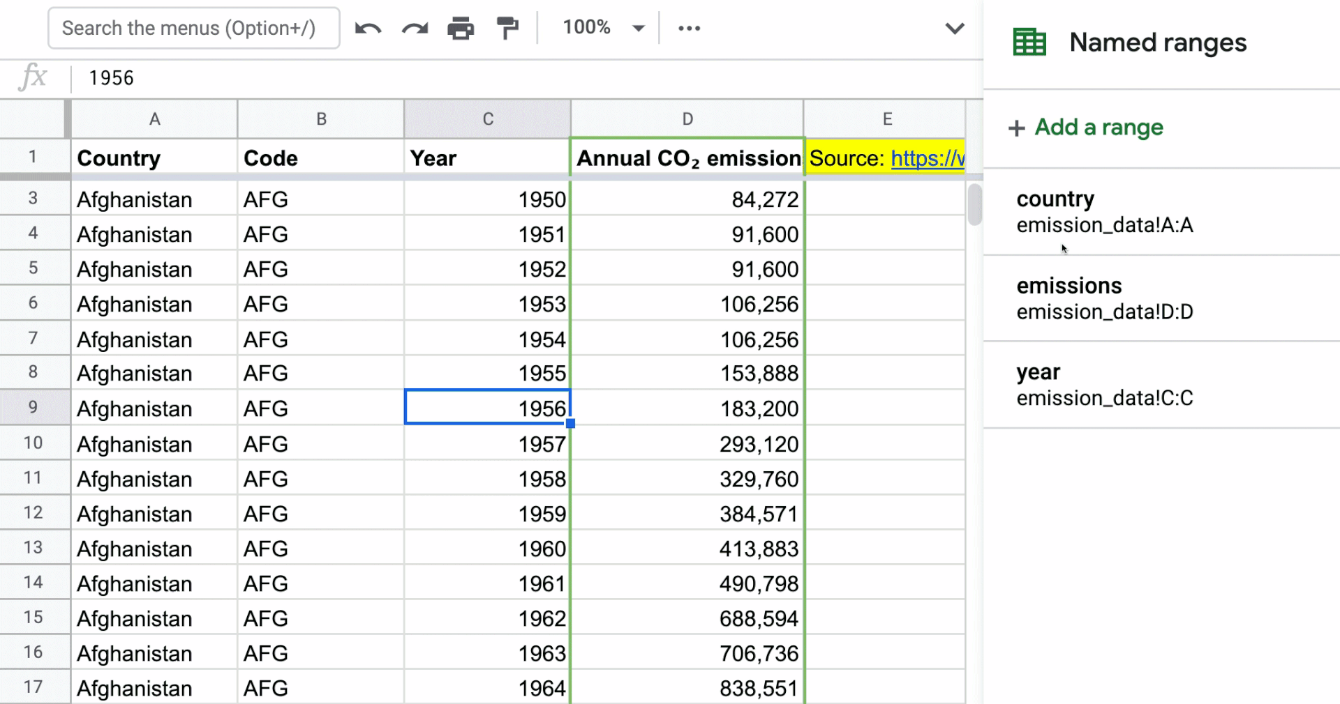
The data set simply looks at all CO₂ emissions for every country by year (in some cases going back to the 1800s). Not quite sure how Our World In Data was able to get data going back this far, but it’s there. The data set consists of four columns and is denormalized (just one long stats table):

About a year ago, National Geographic released a report card on how various countries are tracking towards emissions targets following the Paris Agreement a few years earlier. National Geographic put a few countries in the following buckets: “Top of the class,” “Shows some promise,” and “Barely trying”:

Our raw data set has emission data for every country in the world, and our goal is to build a simply model that outputs the emissions for a few select countries for let’s say the most recent 10 years of data. With this summary data set, we can then start looking at trends, growth patterns, and more. Basically, how do we get something that looks like this (and we can plug in whatever country we want in the first column)?

Modeling with named ranges vs. PivotTables

Since we have a denormalized data set, the easiest way to get the data into the “summary” table structure in the screenshot above is do a PivotTable:

You can play with the filters for Year and Country to just show the data you want. As much as I like PivotTables, it’s not easy to manipulate when you want to change the filters on the fly, so instead we can create a separate summary table that references the raw data using formulas. This is where named ranges come into play.

Applying named ranges to columns in the data set

This is a new technique that I haven’t done before in my models when I was more actively building models, but you’ll see the flexibility once you see how named ranges can work with the Filter function. In the gif below, I’ve named the Country, Year, and Annual CO₂ emissions columns. The named range just represents the entire column. You can access named ranges by going to the “Data” menu in the toolbar.

Referencing named ranges in summary table

Back on the “Model” spreadsheet, I have my countries broken out into the three buckets listed in the National Geographic article. This is a screenshot of the summary table I need to fill out:

Since I have the country in column C and years from columns D onward, I can write a formula to pull in the data I need from the raw emissions data to fill out the table. Here’s what that formula looks like:

Let’s break down why this formula works.

Use of INDIRECT

The INDIRECT function references column A and column A just has the word “emissions” copied down the column. INDIRECT is able to take whatever text you have in a cell and “convert” it to a cell reference. Remember how we made “emissions” a named range in our data set? This INDIRECT function is telling Google Sheets to take column D from our raw data set and turn it into the data we want to reference in this formula.

Another advantage of using INDIRECT in this scenario is that you may have other data sets you want to pull into your main summary table. Let’s say you had population data or energy data for these countries. You would name those columns just like you named the “emissions” column and put the words “population” and “energy” in column A so that Google Sheets knows which data you would like to filter.

Use of FILTER

The FILTER function sits outside as the main function and the first argument it takes is in the actual data you’re trying to filter. In this case, it’s just our emissions data (referenced by using the INDIRECT function). The rest of the arguments are how you actually want to filter your data.

Remember how we also applied named ranges to Year and Country in our raw data? We can now tell the FILTER formula to filter these named ranges (e.g. columns) by the actual year and country in our summary table. Then by using absolute and relative references on our year and country references on the summary table, we can quickly fill the rest of the summary table.

This can be done with GETPIVOTDATA in a PivotTable

Returning back to PivotTables, this summary table could’ve been filled out by referencing a PivotTable as well. Those of you using PivotTables in Excel are probably very familiar with the GETPIVOTDATA function. You could build a PivotTable off of the raw data set, and then use the GETPIVOTDATA function on the summary table to output the data you need.

There are pros and cons with this approach. The con is that you have to create this intermediate PivotTable that sits on another sheet just so you can reference it using the GETPIVOTDATA function. The pro is that your PivotTable constantly updates as you make changes to your raw data set, but this functionality already exists with the FILTER function as described above.

Conclusion

I find the FILTER function in conjunction with named ranges as a much more clean solution because there is no intermediate PivotTable and you can reference the columns you want to filter by their actual names versus a column reference. If you have multiple data sets you need to summarize, having many named ranges may complicate your model, but overall I think having unique names for your columns of data makes your model more readable.

Spreadsheet Day

October 17th is National Pasta Day and National Pay Back A Friend Day. It also happens to be Spreadsheet Day because VisiCalc, the first spreadsheet for personal computers, was released on October 17th, 1979. Debra Dalgleish suggested that this day is Spreadsheet Day back in 2010, so this holiday has been going on for 10 years strong!

To celebrate Spreadsheet Day, the MS Excel Toronto meetup group is hosting a special meetup with Excel’s heavy hitters like Bill Jelen (Mr. Excel), Dan Fylstra (creator of VisiCorp and VisiCalc), Rob Collie (Power Pivot creator), and David Monroy (Senior Program Manager for Microsoft Excel). In general, I’ve found the meetup really educational and have learned a few things from their webinars. Celia Alves has done an amazing job with managing this community and meetup.

Other Podcasts & Blog Posts

In the 2nd half of the episode, I talk about some episodes and blogs from other people I found interesting:

• SaaStr Podcast #367: Zoom Head of Global Sales Operations and Enablement Hilary Headlee