Podcast: Play in new window | Download

Subscribe: Spotify | TuneIn | RSS

You may be filtering and sorting a big dataset in a Google Sheet and want to see that dataset in another Google Sheet without having to copying and pasting the data each time the “source” data is updated. To solve this problem, you need to somehow import the data from the “source” worksheet to your “target” worksheet. When the source worksheet is updated with new sales or customers data, your target worksheet gets updated as well. On top of that, the data that shows up in your target worksheet should be filtered so you only see the data that you need and matters to you. The key to doing this is the IMPORTRANGE() function in conjunction with the FILTER() or QUERY() functions. I’ll go over two methods for importing data from another Google Sheet and talk about the pros and cons of each. You can use this “source” Google Sheet as the raw data and see this target Google Sheet which contains the formulas.

Watch a video tutorial of this post/episode below:

Your Google Sheet is your database

No matter which team you work on, at one point or another your main “database” or “source of truth” was some random Google Sheet. This Google Sheet might have been created by someone in your operations or data engineering team. It may be a data dump from your company’s internal database and whether you like it or not, it contains business-critical data and your team can’t operate without it. The Google Sheet might contain customers data, marketing campaign data, or maybe bug report data that is exported from your team’s Jira workspace.

The reasons why people default to using Google Sheets as their “database” is because anyone can access it in their browser, and more importantly, you can share that Sheet easily with people as long as you have their email address. This is probably your security team’s worst nightmare, but at this point too many teams rely on this Google Sheet so it’s hard to break away from it as a solution.

Credit card customer data

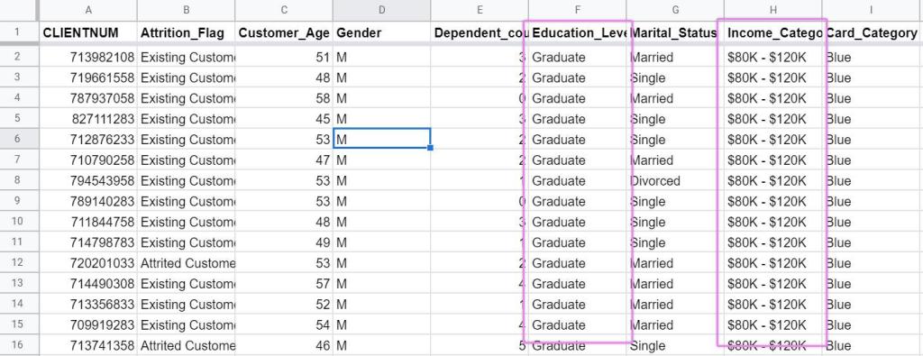
Before we get into the solution, let’s take a look at our data set. Our “source” dataset is a bunch of credit card customer data (5,000 rows) with a customer’s demographic and credit card spending data:

There are a ton of columns in this dataset I don’t care about. I also only want to see the rows where the Education_Level is “Graduate” and the Income_Category is “$80K-$120K.” Perhaps I’m doing an analysis on credit card customers who are high earners and have graduated some college. How do I get that filtered data of graduates earning $80K-$120K into this “target” Sheet:

Google Sheets is not the most ideal solution as a database, but you gotta live with it so let’s see how we can get the data we need from our source Google Sheet over to the target. The money function is IMPORTRANGE() but there are multiple ways of using IMPORTRANGE() as I describe below.

Method 1: The long way with FILTER() and INDEX()

When you use the IMPORTRANGE() function on its own, you will just get all the data from your source Sheet into your target Sheet. In this formula below, I just get all the data from columns A:U in my source Sheet with all the credit card customer data:

The first parameter can be the full URL of the Google Sheet but you can also just get the Sheet ID from the URL to make the formula shorter. The 2nd parameter are the columns you want to pull into your target Sheet.

Again, this will basically give you an exact copy of the source Sheet into your current Sheet. When data is updated in the source, your target Sheet gets updated too. For a lot of scenarios this might be all you need! But let’s go further and try to get a filtered dataset from the source Sheet.

The first thing you’ll probably think of is to use the FILTER() function. The question is what do we put for the second parameter in the FILTER() function?

The first parameter we’ll just use our IMPORTRANGE() function but the second parameter we need to filter by the column that we’re interested in with something like this to get only the rows where the Education_Level is “Graduate”:

=filter(importrange("1H5JljkscteL2qRMJ8ky342uTeP839jjDGg81c8Eg0es","A:U"), F:F="Graduate")

This doesn’t work because F:F is referencing the current worksheet. Our dataset is pulling from a different worksheet and there’s no way to filter that source before it gets into our current worksheet.

The solution is to use the INDEX() function with the FILTER() function like this:

=filter(importrange("1H5JljkscteL2qRMJ8ky342uTeP839jjDGg81c8Eg0es","A:U"),index(importrange("1H5JljkscteL2qRMJ8ky342uTeP839jjDGg81c8Eg0es","A:U"),0,6)="Graduate")

This INDEX() function is telling Google Sheets to look at the source data and focus on the 6th column and see which rows have “Graduate” in them.

We want to filter the data that not only has “Graduate” as the education level but also customers who have a salary of “$80K-$120K.” We can just add additional conditions to our FILTER() formula using this INDEX() trick:

=filter(importrange("1H5JljkscteL2qRMJ8ky342uTeP839jjDGg81c8Eg0es","A:U"),index(importrange("1H5JljkscteL2qRMJ8ky342uTeP839jjDGg81c8Eg0es","A:U"),0,6)="Graduate",index(importrange("1H5JljkscteL2qRMJ8ky342uTeP839jjDGg81c8Eg0es","A:U"),0,8)="$80K - $120K")

We know have a filtered list of about 300 rows:

Pros and cons of this method

The main benefit of this method is that it’s using functions that you may already be familiar with. The main trick is to know how to use the INDEX() function within the FILTER() function.

There are several cons to this method which is why I wouldn’t recommend it (especially if you have a large dataset). Just from filtering two columns, you have to run the IMPORTRANGE() function twice! Imagine filtering on 10 columns. There has got to be a more scalable method than having to nest the IMPORTRANGE() function multiple times in the FILTER() function. This method will definitely get slow over time for large datasets.

Another downside is you can’t control the number of columns that gets returned. Our source data has 21 columns and all 21 get returned. What’s the point of filtering your dataset if you can’t filter the columns that get returned too? You’ll end up hiding a bunch of columns that don’t matter for you in your target worksheet which doesn’t feel right.

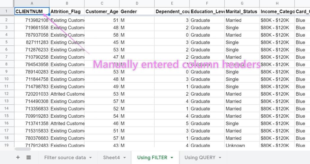
Finally, the column headers in this method are manually entered. Our formula in this method actually gets entered in cell A2 to allow us to copy/paste the column headers into row 1. This means if new columns get added to the source data, you’ll have to remember to add those column headers in your target worksheet. Also not the best method in terms of maintaining this Google Sheet long-term:

Method 2 (preferred): Using QUERY() with a little bit of SQL

The QUERY() function is a relatively advanced function in Google Sheets. Episode 32 was all about how to use the QUERY() function. The reason why it’s not used as much is because it requires you to know a little bit of SQL. To filter our source data to the customers who are “Graduates” and earn “$80K-$120K,” the formula looks like this:

=query(importrange("1H5JljkscteL2qRMJ8ky342uTeP839jjDGg81c8Eg0es","A:U"),"SELECT Col1,Col3,Col6,Col7,Col8,Col9 WHERE Col6='Graduate' and Col8='$80K - $120K'",1)

Just like the FILTER() function, our IMPORTRANGE() is the first parameter. The second parameter is where we have to do a little SQL magic to pull the data we need. All those columns after the SELECT clause are simply the columns we want to pull into our target sheet. This already makes this method more powerful than the first method because we can specify which columns we want from our source Google Sheet. Usually when you use the QUERY() function, you can reference the column by referring to the column letter. With IMPORTRANGE() you have to use the “Col” prefix.

After that, you add in the conditions after the WHERE clause. The trick here is to count the number of columns you want to filter on. In this case, “Col6” is Education_Level and “Col8” is Income_Category.

What’s that last “1” before the closing parentheses? That just tells Google Sheets that our source data has headers so we can pull back our filtered data and the relevant column names. We now get this nice filtered dataset with only the columns we care about:

Pros and cons of this method

In addition to being a much shorter formula, the QUERY() function will bring in the column names. This means you can enter the formula in cell A1 of your target Google Sheet and the data and column names will dynamically update as the source data changes. This means you never have to worry about copying and pasting the column names from the source Google Sheet. This means long-term maintenance of your target Sheet will be much easier.

The main cons:

• QUERY() is a hard function to learn. Learning a new syntax is difficult so if you want to do more advanced filtering and sorting with QUERY() you’ll have to learn more SQL.
• Column numbers can change. This also exists with the first method, but you’ll have to keep track of the column numbers in the source Google Sheet. If new columns get added, you’ll have to adjust your SELECT clause to “pick” the right columns to pull into your target Google Sheet

Final words on using Google Sheets are your database

I could spend another episode on the pros and cons of using Google Sheets as your team or company’s database, but will try to keep my final words short.

Those who don’t use Google Sheets and Excel every day cringe when they see workarounds like this to get the data that we need. The sooner one accepts that business-critical data will inevitably land in an Excel file or Google Sheet, the sooner we can get our jobs done. I’ve written about the unconventional use cases of spreadsheets before and this scenario is no different.

We know our database lives in a Google Sheet. That’s not going to change. Let’s just try to find the most painless way of getting that data out into another Sheet so we can do the more interesting analyses that matter for our business. If you care about the data living in a database and analysts being able to query the data using a separate BI tool, then you should probably consider getting into data engineering and be the change agent within your organization to move everyone off of spreadsheets. It’s a gargantuan task and in most cases an uphill battle.

Other Podcasts & Blog Posts

In the 2nd half of the episode, I talk about some episodes and blogs from other people I found interesting:

• Making Sense Podcast: Special Episode – Engineering The Apocalypse